Input manipulation with pre-trained models
The robustness library provides functionality to perform various input space manipulations using a trained model. This ranges from basic manipulation such as creating untargeted and targeted adversarial examples, to more advanced/custom ones. These types of manipulations are precisely what we use in the code releases for our papers [EIS+19] and [STE+19].
Download a Jupyter notebook containing all the code from this walkthrough!Generating Untargeted Adversarial Examples
First, we will go through an example of how to create untargeted adversarial examples for a ResNet-50 on the dataset CIFAR-10.
Load the dataset using:
import torch as ch
from robustness.datasets import CIFAR
ds = CIFAR('/path/to/cifar')
Restore the pre-trained model using:
from robustness.model_utils import make_and_restore_model
model, _ = make_and_restore_model(arch='resnet50', dataset=ds,
             resume_path=PATH_TO_MODEL)
model.eval()
Create a loader to iterate through the test set (set hyperparameters appropriately). Get a batch of test image-label pairs:
_, test_loader = ds.make_loaders(workers=NUM_WORKERS,
                                    batch_size=BATCH_SIZE)
_, (im, label) = next(enumerate(test_loader))
Define attack parameters (see
robustness.attacker.AttackerModel.forward()for documentation on these parameters):kwargs = { 'constraint':'2', # use L2-PGD 'eps': ATTACK_EPS, # L2 radius around original image 'step_size': ATTACK_STEPSIZE, 'iterations': ATTACK_STEPS, 'do_tqdm': True, }
The example considers a standard PGD attack on the cross-entropy loss. The parameters that you might want to customize are
constraint('2'and'inf'are supported),'attack_eps','step_size'and'iterations'.Find adversarial examples for
imfrom step 3:_, im_adv = model(im, label, make_adv=True, **kwargs)
If we want to visualize adversarial examples
im_advfrom step 5, we can use the utilities provided in therobustness.toolsmodule:from robustness.tools.vis_tools import show_image_row from robustness.tools.label_maps import CLASS_DICT # Get predicted labels for adversarial examples pred, _ = model(im_adv) label_pred = ch.argmax(pred, dim=1) # Visualize test set images, along with corresponding adversarial examples show_image_row([im.cpu(), im_adv.cpu()], tlist=[[CLASS_DICT['CIFAR'][int(t)] for t in l] for l in [label, label_pred]], fontsize=18, filename='./adversarial_example_CIFAR.png')
Here is a sample output visualization snippet from step 6:
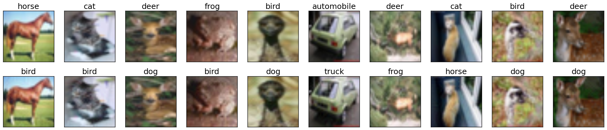
Random samples from the CIFAR-10 test set (top row), along with their corresponding untargeted adversarial examples (bottom row). Image titles correspond to ground truth labels and predicted labels for the top and bottom row respectively.
Generating Targeted Adversarial Examples
The procedure for creating untargeted and targeted adversarial examples using the robustness library are very similar. In fact, we will start by repeating steps 1-3 describe above. The rest of the procedure is as follows (most of it involves minor modifications to steps 4-5 above):
Define attack parameters:
kwargs = {
    'constraint':'2',
    'eps': ATTACK_EPS,
    'step_size': ATTACK_STEPSIZE,
    'iterations': ATTACK_STEPS,
    'targeted': True,
    'do_tqdm': True
}
The key difference from step 4 above is the inclusion of an additional parameter
'targeted'which is set toTruein this case.Define target classes towards which we want to perturb
im. For instance, we can perturb all the images towards class0:targ = ch.zeros_like(label)
Find adversarial examples for
im:_, im_adv = model(im, targ, make_adv=True, **kwargs)
If you would like to visualize the targeted adversarial examples, you can repeat
the aforementioned step 6, i.e. the
robustness.tools.vis_tools.show_image_row() method:
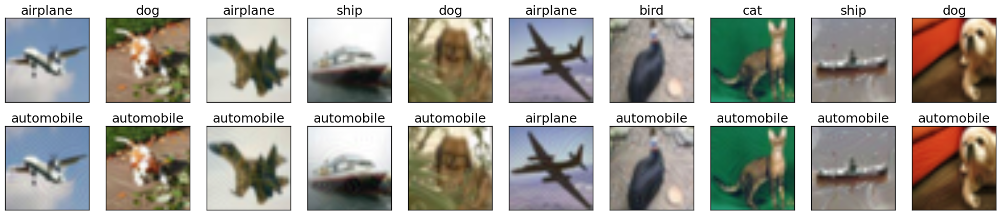
Random samples from the CIFAR-10 test set (top row), along with their corresponding targeted adversarial examples (bottom row). Image titles correspond to ground truth labels and predicted labels (target labels) for the top and bottom row respectively.
Custom Input Manipulation (e.g. Representation Inversion)
You can also use the robustness lib functionality to perform input
manipulations beyond adversarial attacks. In order to do this, you will need to
define a custom loss function (to replace the default
ch.nn.CrossEntropyLoss).
We will now walk through an example of defining a custom loss for inverting the representation (output of the pre-final network layer, before the linear classifier) for a given image. Specifically, given the representation for an image, our goal is to find (starting from noise) an input whose representation is close by (in terms of euclidean distance).
First, we will repeat steps 1-3 from the procedure for generating untargeted adversarial examples.
Load a set of images to invert and find their representation. Here we choose random samples from the test set:
_, (im_inv, label_inv) = next(enumerate(test_loader)) # Images to invert
with ch.no_grad():
    (_, rep_inv), _ = model(im_inv, with_latent=True) # Corresponding representation
We now define a custom loss function that penalizes difference from a target representation
targ:def inversion_loss(model, inp, targ): # Compute representation for the input _, rep = model(inp, with_latent=True, fake_relu=True) # Normalized L2 error w.r.t. the target representation loss = ch.div(ch.norm(rep - targ, dim=1), ch.norm(targ, dim=1)) return loss, None
We are now ready to define the attack args :samp: kwargs. This time we will supply our custom loss
inversion_loss:kwargs = { 'custom_loss': inversion_loss, 'constraint':'2', 'eps': 1000, 'step_size': 1, 'iterations': 10000, 'targeted': True, 'do_tqdm': True, }
We now define a seed input which will be the starting point for our inversion process. We will just use a gray image with (scaled) Gaussian noise:
im_seed = ch.clamp(ch.randn_like(im_inv) / 20 + 0.5, 0, 1)
Finally, we are ready to perform the inversion:
_, im_matched = model(im_seed, rep_inv, make_adv=True, **kwargs)
We can also visualize the results of the inversion process (similar to step 6 above)::
show_image_row([im_inv.cpu(), im_seed.cpu(), im_matched.cpu()],
         ["Original", r"Seed ($x_0$)", "Result"],
         fontsize=18,
         filename="./custom_inversion_CIFAR.png")
You should see something like this:
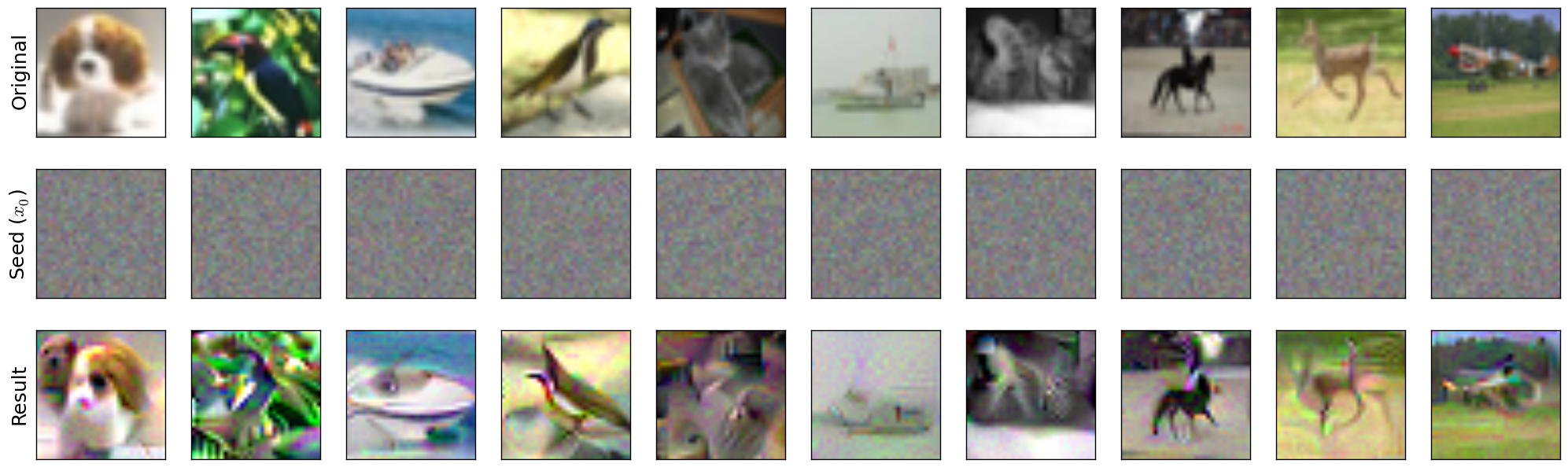
Inverting representations of a robust network. Starting from the seed (middle row), we optimize for an image (bottom row) that is close to the representation of the original image (top row).
Changing optimization methods
In the above, we consistently used L2-PGD for all of our optimization tasks, as
dictated by the value of the constraint argument to the model. However,
there are a few more possible optimization methods available in the
robustness package by default. We give a brief overview of them here—the
robustness.attack_steps module has more in-depth documentation on each
method:
- If
kwargs['constraint'] == '2'(as it was for this walkthrough), thenepsis interpreted as an L2-norm constraint, and we take \(\ell_2\)-normalized gradient steps. More information atrobustness.attack_steps.L2Step. - If
kwargs['constraint'] == 'inf', thenepsis interpreted as an \(\ell_\infty\) norm constraint, and we take \(\ell_\infty\)-normalized PGD steps (i.e. signed gradient steps). More information atrobustness.attack_steps.LinfStep. - If
kwargs['constraint'] == 'unconstrained', thenepsis ignored and the adversarial image is only clipped to the [0, 1] range. The optimization method is ordinary gradient descent, i.e., no projection is done to the gradient before making a step. - If
kwargs['constraint'] == 'fourier', thenepsis ignored and the adversarial image is only clipped to the [0, 1] range. The optimization method is once again ordinary gradient descent, but this time in the Fourier basis rather than the pixel basis. This tends to yield nicer-looking images, for reasons discussed here [OMS17].
For example, in order to do representation inversion in the fourier basis rather
than the pixel basis, we would change kwargs as follows:
kwargs = {
    'custom_loss': inversion_loss,
    'constraint':'fourier',
    'eps': 1000, # ignored anyways
    'step_size':  5000, # have to re-tune LR
    'iterations': 1000,
    'targeted': True,
    'do_tqdm': True,
}
We also have to change our im_seed to be a valid Fourier-basis
parameterization of an image:
im_seed = ch.randn(BATCH_SIZE, 3, 32, 32, 2) / 5 # Parameterizes a grey image
Running this through the model just like before and visualizing the results should yield something like:
show_image_row([im_inv.cpu(), im_matched.cpu()],
      ["Original", "Result"],
      fontsize=18,
      filename='./custom_inversion_CIFAR_fourier.png')
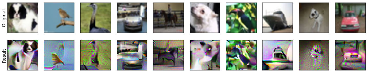
Inverting representations of a robust network in the fourier basis. Starting from the seed (middle row), we optimize for an image (bottom row) that is close to the representation of the original image (top row).
Below we show how to implement our own custom optimization methods as well.
| [OMS17] | Olah, et al., “Feature Visualization”, Distill, 2017. |
Advanced usage
The steps given above are sufficient for using the robustness library
for a wide a variety of input manipulation techniques, and for reproducing the
code for our papers. Here we go through a couple more advanced options and
techniques for using the library.
Gradient Estimation/NES
The first more advanced option we look at is how to use estimated gradients
in place of real ones when doing adversarial attacks (this corresponds to the
NES black-box attack [IEA+18]). To do this, we simply need to provide the
est_grad argument (None by default) to the model upon creation of the
adversarial example. As discussed in this docstring, the proper format for this argument is
a tuple of the form (R, N), and the resulting gradient estimator is
where \(\delta_i\) are randomly sampled from the unit ball (note that we employ antithetic sampling to reduce variance, meaning that we actually draw \(N/2\) random vectors from the unit ball, and then use \(\delta_{N/2+i} = -\delta_{i}\).
To do representation inversion with NES/estimated gradients, we would just need to add the following line to the above:
kwargs['est_grad'] = (0.5, 100)
This will run the optimization process using 100-query gradient estimates with \(R = 0.5\) in the above estimator.
| [IEA+18] | Ilyas, A., Engstrom, L., Athalye, A., & Lin, J. (2018). Black-box adversarial attacks with limited queries and information. arXiv preprint arXiv:1804.08598. |
Custom optimization methods
To make a custom optimization method, all that is required is to subclass
robustness.attack_steps.AttackerStep class. The class documentation has
information about which methods and properties need to be implemented, but
perhaps the most illustrative thing is an example of how to implement the
\(\ell_2\)-PGD attacker:
class L2Step(AttackerStep):
   def project(self, x):
      diff = x - self.orig_input
      diff = diff.renorm(p=2, dim=0, maxnorm=self.eps)
      return ch.clamp(self.orig_input + diff, 0, 1)

   def step(self, x, g):
      # Scale g so that each element of the batch is at least norm 1
      l = len(x.shape) - 1
      g_norm = ch.norm(g.view(g.shape[0], -1), dim=1).view(-1, *([1]*l))
      scaled_g = g / (g_norm + 1e-10)
      return x + scaled_g * self.step_size

   def random_perturb(self, x):
      new_x = x + (ch.rand_like(x) - 0.5).renorm(p=2, dim=1, maxnorm=self.eps)
      return ch.clamp(new_x, 0, 1)

   def to_image(self, x):
      return x
As part of initialization, the properties self.orig_input, self.eps, and
self.step_size, and self.use_grad will already be defined. As shown
above, there are four functions that your custom step can implement (three of
which, project, step, and random_perturb, are mandatory).
- The
projectfunction takes in an inputxand projects it to the appropriate ball aroundself.orig_input. - The
stepfunction takes in a current input and a gradient, and outputs the next iterate of the optimization process (in our case, we normalize the gradient and then add it to the iterate to perform an \(\ell_2\) projected gradient ascent step). - The
random_perturbfunction is called if therandom_startoption is given when constructing the adversarial example. Given an input, it should apply a small random perturbation to the input while still keeping it within the adversarial budget. - The
to_imagefunction is identity by default, but is useful when working with alternative parameterizations of images. For example, when optimizing in Fourier space, theto_imagefunction takes in an input which is in the Fourier basis, and outputs a valid image.